Nbodyplot Class

This module provides the basic functions to plot the simulation of a N-body problem. This module is based on matplotlib.

Build a Nbodyplot object

plt = nbodypy.Nbodyplot()

Here the documentation of the constructor.

Nbodyplot.__init__(fig=1)

Constructor :param fig: (int) number of the matplotlib figure we consider (default =1)

One can define multiple plots using the optional parameter fig.

Plot a solution

Plot a 2 dimensional solution

Nbodyplot.plotSol2D(nbody, t, mode='show', name='trajectory', boundingbox=None)

Plot trajectory in the (x,y)-plane

Parameters:

• nbody – Nbody Class Instance
• t – (numpy.array) array of times of integration to plot the solution
• mode – (str) to chose if window show or print in a ‘pdf’ or ‘png’ file (default ‘show’)
• name – (str) name of the file if png or pdf file is generated (default ‘trajectory’)
• boundingbox – (list) of the form [xmin xmax ymin ymax] (default None)

Let us plot a 2 dimensional system (that is to say with a dim parameter equal to two).

plt = nbodypy.Nbodyplot()
zinit = numpy.array([0, 0.316046051487446, 0.864077674448677, 0,  0.100941149773621, -0.158023025743723, -0.432038837224337, 2.02906597904133, -0.100941149773621 , -0.158023025743723,  -0.43203883722434, -2.02906597904133])

Eight = nbodypy.Nbody(N=3,init=zinit)
t = numpy.linspace(0, 1.0/3, 100)
plt.plotSol2D(Eight,t, mode="png",name="Eight")

This example produce a png file.

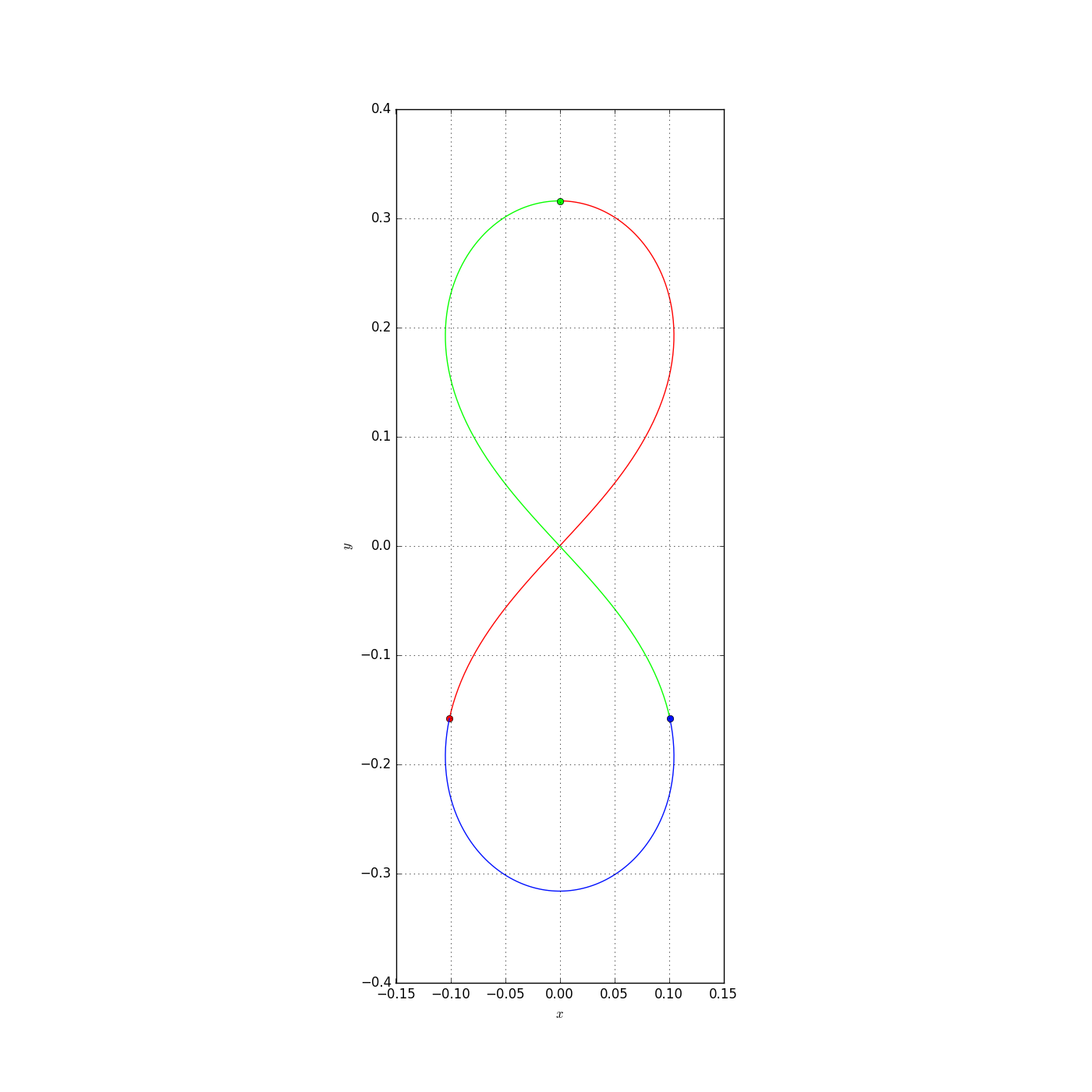
The first parameter is an instance of the Nbody class, the second is an numpy.array of times to plot the solution.

The mode parameter allows to choose the mode of representation. By default, we have a popup window, produced by matplotlib, in which the figure is plotted. We can choose png or pdf to produce external file.

The boundingbox allows to chose the bounding box of the plot in the local coordinates, by default (None), the bounding box is automatically computed by matplotlib.

Plot a 3 dimensional solution

Nbodyplot.plotSol3D(nbody, t, mode='show', name='trajectory', projection=True)

Plot trajectory in the (x,y)-plane, (y,z)-plane, (x-z)-plane and 3D view

Parameters:

• nbody – Nbody Class Instance
• t – (numpy.array) time of integration to plot the solution
• mode – (str) to chose if window show or print in a ‘pdf’ or ‘png’ file (default ‘show’)
• name – (str) name of the file if png or pdf file is generated (default ‘trajectory’)
• projection – (boolean) to choose if we want 2D projections (on (x,y)-plane, (y,z) plane and (x,z)-plane, default) or to choose a 3D visualization

plt = nbodypy.Nbodyplot()

zinit = numpy.array([0.165649854848924,  3.0549363634996e-151 ,    0.209141794901608,
                  8.86909514289322e-29 ,     2.03225904939571, -9.31938237331704e-29,
                  -0.0828249274244622 ,    0.160070428973807,    -0.104570897450804,
                  -2.04906075007578 ,    -1.01612952469786 ,     1.15731474026243,
                  -0.0828249274244618 ,   -0.160070428973807 ,   -0.104570897450804,
                  2.04906075007578,     -1.01612952469785,     -1.15731474026243])

Arotating = numpy.array([[0.0, 5.13873206001209, 0.0],
                      [-5.13873206001209, 0.0, 0.0],
                      [0.0,0.0, 0.0]])



Rotating3D = nbodypy.Nbody(N=3, dim=6, init = zinit,rotating=Arotating)
t = numpy.linspace(0, 1.0/3.0, 100)
plt.grid = False
plt.points = True
plt.plotSol3D(Rotating,t,mode='png',name="Rotating")

This example produce the following picture.

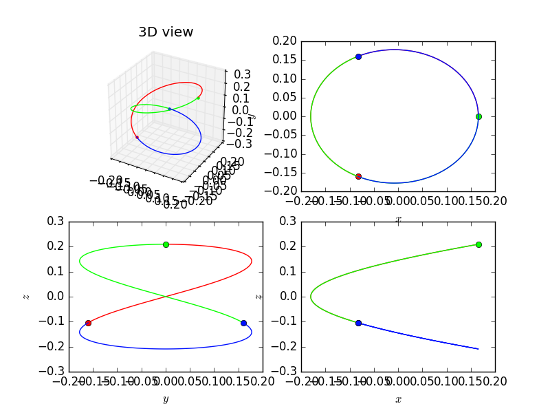
The default parameter projection is equal to True. If we set it to False then we obtain only the 3D view.

Plot a 4 dimensional solution

Nbodyplot.plotSol4D(nbody, t, mode='show', name='trajectory', projection='3d')

Plot a four dimensional solution

Parameters:

• nbody – Nbody Class Instance
• t – (float) time of integration to plot the solution (numpy.array)
• mode – (str) to chose if window show or print in a ‘pdf’ or ‘png’ file (default ‘show’)
• name – (str) name of the file if png or pdf file is generated (default ‘trajectory’)
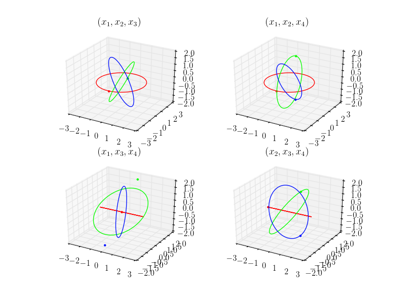
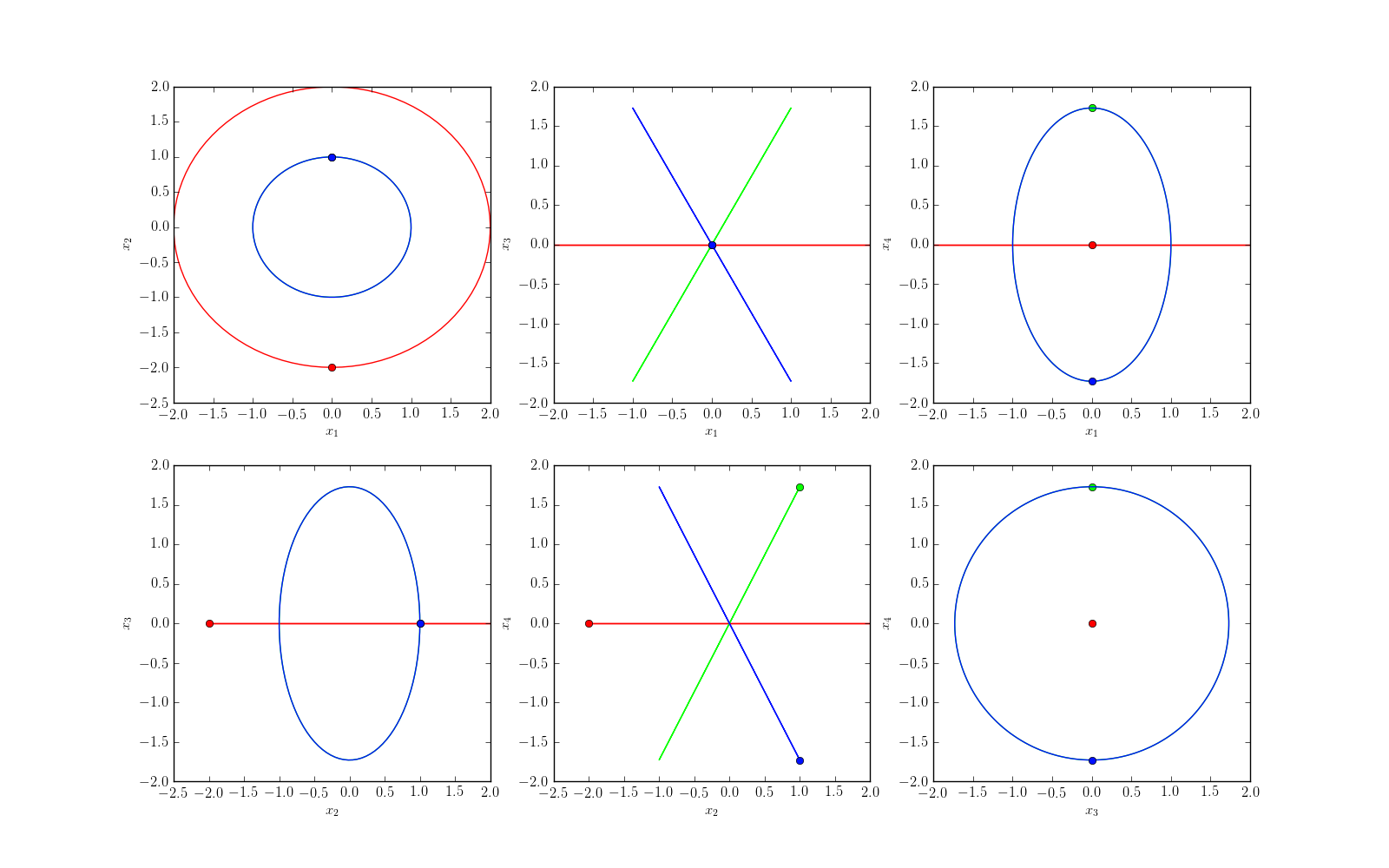
• projection – (string) to choose, ‘3d’ (default) : trajectories in the (x1,x2,x3)-plane, (x1,x2,x4)-plane, (x1,x3,x4)-plane, (x2,x3,x4)-plane,‘2d’: trajectories in the (x1,x2)-plane, (x1,x3)-plane, (x1,x4)-plane, (x2,x3)-plane, (x2,x4)-plane, (x3,x4)-plane

plt = nbodypy.Nbodyplot()
plt.points = True

Ortho4D = nbodypy.Nbody(jsonFile="4DExample.json")
t = numpy.linspace(0, 23.388651110001, 100)

plt.plotSol4D(Ortho4D,t,mode='png',name="Ortho4D")

This example produce the following picture.

We can plot the solution using 2D projections. For that, we set the parameter projection to 2d.

plt = nbodypy.Nbodyplot()
plt.points = True

Ortho4D = nbodypy.Nbody(jsonFile="4DExample.json")
t = numpy.linspace(0, 23.388651110001, 100)

plt.plotSol4D(Ortho4D,t,mode='png',projection='2d',name="Ortho4D2d")

Make movies

Nbodyplot.CreateMovie2D(nbody, time, numberOfFrames, prevTime=0.0, fps=24, name='trajectory', keep=False, mode='png', boundingbox=None)

Function to create a movie of the plot of a 2D solution. The fuction produce a set of pictures that may be collected to build a video with avconv software.

Parameters:

• nbody – Nbody Class Instance
• time – (float) total time of integration
• numberOfFrames – (int) number of Frames for the total video
• prevTime – (float) to get a trace of the past of each body (defaults 0.0)
• fps – (int) frame per second (default 24)
• keep – (boolean) to keep the different generated images (default False)
• mode – (str) to choose the format of each generated image (default ‘png’), if mode=’png’ a mp4 movie is created
• boundingbox – (list) of the form [xmin xmax ymin ymax] (default None)

Here is an example of the use of this method.

plt = nbodypy.Nbodyplot()

zinit = numpy.array([0, 0.316046051487446, 0.864077674448677, 0,  0.100941149773621, -0.158023025743723, -0.432038837224337, 2.02906597904133, -0.100941149773621 , -0.158023025743723,  -0.43203883722434, -2.02906597904133])

Eight = nbodypy.Nbody(N=3,init=zinit)
t = numpy.linspace(0, 1.0/3, 100)
Eight.integrate(t,fileName="fileEight")
plt.CreateMovie2D(Eight,1.0,200,prevTime=1.0/3, name="Eight",boundingbox=[-0.20,0.20,-0.4,0.4])

which produce a video numed `movieEight.mp4”.

You can produce other types of images such as svg, jpg, pdf, but the movie creation is only possible with the png mode. To create a video, you have to install the aconv software (avaliable on linux at least).

The CreateMovie2D method use the following intern method:

Nbodyplot.imageMovie2D(nbody, sol, I, prevIt=0, boundingbox=None)

Function to create a image of the plot of a 2D solution to create a film

Parameters:

• nbody – Nbody Class Instance
• sol – (numpy.array) output of nbodypy.integrate() function
• I – (int) current, the range in the sol array
• prevIt – (int) the previous range in the sol array, depending on the rate and the size of sol
• boundingbox – (list) of the form [xmin xmax ymin ymax] (default None)

Parameters for the plots

There is two parameters:

• the grid one with the True default value and that allows to draw a grid behind the trajectories or not.
• The points parameter with the True default value and that allows to draw bullets to mark the bodies.